Step-by-Step Guide to Data Manipulation in Python

In 2025, global data creation has reached an all-time high. According to IDC, the total amount of digital data created worldwide is projected to surpass 175 zettabytes, driven by IoT, cloud platforms, AI systems, and real-time analytics. Organizations now generate over 2.5 quintillion bytes of data every day, and this trend is only accelerating.

But here’s the catch: raw data is rarely useful in its original form. Before data scientists or analysts can extract insights, they must first manipulate the data—clean it, reshape it, join it, and prepare it for modeling or decision-making. This process is called data manipulation, and it lies at the very foundation of modern data science.

Python is the most popular language for this task, thanks to its simplicity and powerful libraries like Pandas, NumPy, and Dask.

What is Data Manipulation?

Data manipulation refers to the process of adjusting data to make it organized and easier to read or analyze. This includes cleaning, structuring, aggregating, and transforming data to fit specific purposes or formats. For example, raw survey data collected from users might need to be filtered, normalized, and formatted before it can be visualized or used in machine learning.

Without proper data manipulation, decisions based on the data can be inaccurate or misleading. Thus, understanding how to manipulate data efficiently is crucial for professionals in analytics, business intelligence, and data science roles.

Key Python Libraries for Data Manipulation

Python’s strength in data manipulation lies in its diverse and mature ecosystem of libraries. Each library is tailored to handle specific types of data operations—from basic numerical tasks to complex distributed processing. Here are the most essential Python libraries for data manipulation in 2025

1. Pandas

Pandas is the cornerstone of data manipulation in Python. It introduces DataFrames and Series—data structures that allow easy handling of structured data. Whether you're loading CSVs, cleaning tables, or performing statistical operations, Pandas is likely your go-to tool. It offers functions for indexing, filtering, merging, reshaping, and aggregating data.

Key capabilities include:

• Handling missing data

• GroupBy operations

• Merging/joining datasets

• Time series functionality

• Reading/writing to various formats (CSV, Excel, SQL, JSON)

Pandas is designed to be user-friendly, making it accessible even for beginners in data science.

2. NumPy

NumPy, short for Numerical Python, is the foundational package for numerical computing in Python. It provides fast and memory-efficient array structures called ndarrays, and is often used under the hood by libraries like Pandas and Scikit-learn.

NumPy is excellent for tasks like:

• Element-wise mathematical operations

• Broadcasting and vectorization

• Linear algebra computations

• Statistical analysis

Its performance and speed make it ideal for large-scale scientific and engineering calculations.

3. OpenPyXL and xlrd

For projects that involve Excel files, OpenPyXL and xlrd are indispensable. These libraries allow Python users to read, write, and manipulate Excel spreadsheets (.xlsx, .xls). OpenPyXL is preferred for modern Excel formats and supports rich formatting, charts, and formula parsing.

Common use cases include:

• Automating Excel reports

• Reading financial models

• Cleaning spreadsheet exports from business tools

4. CSV

The csv module is a built-in Python library for reading and writing CSV files. While it lacks the advanced functionality of Pandas, it’s useful for quick file manipulations when dependencies must be kept minimal.

It’s often used for:

• Lightweight parsing of CSVs

• Scripting small data processing tasks

  
  

• Exporting structured data

5. Dask and Vaex

As datasets grow larger than memory, traditional libraries like Pandas may struggle. That’s where Dask and Vaex come in. They provide scalable, parallelized alternatives for working with massive datasets.

• Dask mirrors the Pandas API and enables distributed computing across multiple cores or even clusters.

• Vaex is optimized for lazy loading and out-of-core processing, allowing fast exploration of billions of rows.

These libraries are crucial for big data workflows in finance, healthcare, and cloud-native applications.

Each of these libraries brings unique strengths to the table. Whether you're working with simple spreadsheets or terabytes of event logs, choosing the right library—and knowing how to use it—can drastically improve your productivity and outcomes in any data-driven project.

Essential Components of Data Manipulation in Python

1. Importing and Reading Data

The very first step in any data workflow involves reading data into Python. Python supports a variety of file formats and sources such as CSV, Excel, JSON, SQL databases, and even remote APIs. Using libraries like Pandas and built-in modules like csv, you can quickly load structured datasets into DataFrames—Pandas’ two-dimensional data structure resembling a spreadsheet.

Example:

import pandas as pd

df = pd.read_csv("sales_data.csv")

Once loaded, you should immediately inspect your dataset. Use functions such as .head() to view the first few rows, .info() for data types and memory usage, and .describe() for statistical summaries. These insights help you understand the structure of your data and identify inconsistencies, missing values, or formatting issues.

If you’re working with Excel, the read_excel() function is your friend. For larger or non-traditional files like JSON, APIs, or SQL tables, Pandas offers corresponding functions such as read_json() or read_sql() to fetch data effortlessly. By mastering these functions, you create a solid foundation for the rest of your data pipeline.

2. Cleaning and Preprocessing Data

Once the data is loaded, the next critical step is cleaning and preprocessing. Raw data often contains missing values, incorrect data types, duplicate entries, or inconsistent formatting. If not addressed, these issues can skew analysis and lead to incorrect conclusions.

Handling Missing Values

Missing data is common in real-world datasets. Depending on the context, you might choose to fill in missing values with defaults, the mean/median, or remove those rows entirely:

# Fill missing values with zero

df.fillna(0, inplace=True)

# Drop rows with any missing values

df.dropna(inplace=True)

You can also use advanced imputation methods using libraries like sklearn.impute if needed for machine learning tasks.

Correcting Data Types

Sometimes, numerical columns are mistakenly interpreted as strings. Or dates are stored as text. Ensuring the correct data type helps avoid errors and supports efficient operations:

# Convert column to numeric

df['amount'] = pd.to_numeric(df['amount'], errors='coerce')

# Convert column to datetime

df['order_date'] = pd.to_datetime(df['order_date'])

Removing Duplicates

Duplicate records can inflate metrics or introduce redundancy. Use the following command to remove them:

df.drop_duplicates(inplace=True)

Renaming Columns

To make your dataset cleaner or more readable, rename columns with meaningful names:

df.rename(columns={'amt': 'amount_usd'}, inplace=True)

Trimming Whitespace and Standardizing Text

Inconsistent capitalization or hidden spaces can make categorical data difficult to analyze:

df['product'] = df['product'].str.strip().str.lower()

By performing these preprocessing steps, your dataset becomes structured, clean, and ready for deeper analysis or visualization.

 3. Filtering and Selecting Data

Once your data is cleaned and structured, the next step is often to filter specific subsets of information or select relevant columns and rows for analysis. Python makes this process highly efficient using Pandas’ built-in methods.

Selecting Columns

You can access a single column in a DataFrame like this:

df['column_name']

To select multiple columns:

df[['column1', 'column2']]

This is useful when preparing a smaller dataset for modeling or visualization.

Filtering Rows Based on Conditions

You can filter rows by defining conditions. For example, if you only want rows where age is greater than 30:

df[df['age'] > 30]

You can also combine multiple conditions using logical operators:

df[(df['age'] > 30) & (df['city'] == 'Pune')]

Using loc and iloc

• loc[] is label-based indexing. It is used to select rows and columns by their labels:

df.loc[0:5, ['name', 'salary']]

• iloc[] is integer-location based indexing:

df.iloc[0:5, 0:2]

These methods provide more control when slicing data for complex manipulations.

Sorting Data

Sorting is essential for organizing data, identifying top values, or preparing for reporting:

df.sort_values(by='salary', ascending=False)

You can sort by one or multiple columns.

Filtering and selection help you focus on the most relevant data and reduce the noise in your analysis. This step is especially crucial when dealing with large datasets or when building dashboards where only key insights are needed.

4. Grouping and Aggregation

Grouping and aggregation are powerful techniques used to summarize and analyze data efficiently. These operations are especially useful when working with large datasets, allowing you to break down data by categories and compute metrics like averages, counts, and sums.

Grouping Data

The groupby() function in Pandas allows you to split your data into groups based on a specific column and then apply an aggregate function:

df.groupby('department')['salary'].mean()

This line of code groups the data by the department column and calculates the average salary in each department.

You can also group by multiple columns:

df.groupby(['department', 'gender'])['salary'].mean()

This lets you compute more granular insights, like average salary by department and gender.

Applying Aggregation Functions

Pandas offers a wide range of aggregation functions like sum(), mean(), count(), min(), and max():

df.groupby('city')['sales'].sum()

df.groupby('city')['sales'].max()

You can also apply multiple aggregation functions at once using the agg() method:

df.groupby('product').agg({'sales': ['sum', 'mean'], 'quantity': 'sum'})

This returns a DataFrame with both the sum and mean of sales and the total quantity sold for each product.

Resetting Index

After a groupby operation, the resulting object has the grouping column as the index. If you prefer a clean DataFrame, use:

grouped_df.reset_index(inplace=True)

This is useful when merging grouped data back into the original dataset or exporting it.

Grouping and aggregation make it easy to analyze trends, compare segments, and summarize performance metrics. These techniques are foundational for reporting and dashboarding tasks.

 5. Merging and Joining Data

In many real-world scenarios, data comes from different sources or files. To get a complete view, it's essential to combine these datasets accurately. Python, through Pandas, provides robust tools for merging and joining datasets based on keys or indexes.

Merging Datasets

The merge() function in Pandas works similarly to SQL joins. You can merge two datasets on a common column:

df_merged = pd.merge(df1, df2, on='id', how='inner')

This performs an inner join, returning rows that have matching keys in both DataFrames. You can also perform left, right, and outer joins:

df_left = pd.merge(df1, df2, on='id', how='left')

df_outer = pd.merge(df1, df2, on='id', how='outer')

Choosing the right type of join depends on your use case—whether you want all records, only matching records, or all records from one dataset.

Concatenating Datasets

If your datasets share the same structure (i.e., same columns), you can stack them vertically using concat():

df_combined = pd.concat([df1, df2], axis=0)

This is especially useful for combining datasets split across time or geography.

To merge datasets side by side (i.e., add columns), you can use:

df_side_by_side = pd.concat([df1, df2], axis=1)

Joining on Index

You can also merge datasets based on their index values:

df_joined = df1.join(df2, how='inner')

This method is simple when your data is already aligned by index.

Handling Duplicates and Conflicts

When merging datasets, you may encounter duplicate columns or conflicting data. Pandas offers parameters like suffixes to resolve such issues:

df_merged = pd.merge(df1, df2, on='id', suffixes=('_left', '_right'))

Merging and joining are critical for building comprehensive datasets that bring together multiple perspectives, be it combining sales with customer details or unifying survey data with transactional records.

 6. Reshaping Data: Pivoting and Melting

Reshaping data refers to changing its structure without modifying its content. This is often required when converting data formats for reporting, analysis, or machine learning tasks. Two of the most powerful techniques in Pandas for reshaping data are pivoting and melting.

Pivoting Data

Pivoting is the process of converting rows into columns. It's useful when you want to reorganize data into a matrix format that makes trends easier to analyze.

df_pivot = df.pivot_table(index='Region', columns='Year', values='Sales', aggfunc='sum')

This example groups the dataset by 'Region' and 'Year' and shows the sum of sales for each combination. It’s a great way to turn long-format data into a cross-tabulated summary.

You can also use pivot() for a simpler version of pivoting if your dataset doesn’t have duplicates:

df.pivot(index='Region', columns='Year', values='Sales')

Melting Data

Melting is the opposite of pivoting. It transforms wide-format data into a long format, which is often preferred for visualization or when passing data to certain machine learning algorithms.

df_melted = pd.melt(df, id_vars=['Region'], value_vars=['2019', '2020', '2021'], var_name='Year', value_name='Sales')

This reshapes the data so each year becomes a row under a single 'Year' column, making it easier to plot or model.

Melting is particularly useful when you receive data in a spreadsheet-style format and need to make it more usable for Pandas or Seaborn.

When to Use Which

• Use pivot when you want to summarize and structure data in a compact table format.

• Use melt when you need a normalized structure that’s easy to filter, group, or visualize.

Understanding pivoting and melting gives you more flexibility in how you store and view your datasets, allowing for customized analysis pipelines and clearer visualizations.

7. Working with Time-Series Data

Time-series data—where observations are indexed in time order—is one of the most common forms of data in domains like finance, weather forecasting, inventory tracking, and web analytics. Python provides robust tools through Pandas to handle time-based data efficiently.

Converting Strings to Datetime

To work with time-series data, ensure your date columns are in a datetime format:

df['order_date'] = pd.to_datetime(df['order_date'])

This conversion unlocks powerful features like time-based indexing, slicing, and resampling.

Extracting Date Components

Once converted, you can easily extract parts of a date for more granular analysis:

df['year'] = df['order_date'].dt.year

df['month'] = df['order_date'].dt.month

df['day'] = df['order_date'].dt.day

These components are useful for time-based aggregations and visualizations.

Time-Based Filtering

You can filter datasets based on specific time windows:

df[df['order_date'] >= '2025-01-01']

This is particularly useful for generating monthly or quarterly reports.

Resampling Time-Series Data

Pandas allows you to resample time-series data to different frequencies:

df.set_index('order_date', inplace=True)

monthly_sales = df['sales'].resample('M').sum()

This command groups data by month and calculates the total sales, ideal for trend analysis.

Rolling Windows

To smooth out fluctuations in time-series data, apply rolling statistics:

df['rolling_avg'] = df['sales'].rolling(window=3).mean()

This computes a moving average over a three-period window, helping to identify trends and seasonality.

Working with time-series data is vital for predictive modeling, business reporting, and understanding historical patterns. With Pandas' datetime capabilities, you can efficiently analyze, visualize, and forecast time-based metrics.

8. Manipulating and Cleaning Textual Data

In real-world datasets, especially those coming from customer feedback, surveys, or social media, textual data plays a critical role. Handling unstructured text requires specific techniques to clean, transform, and analyze it effectively. Python’s Pandas and built-in string functions provide essential tools for text manipulation.

Removing Whitespace and Standardizing Case

Text data often comes with extra spaces or inconsistent casing that can skew results during filtering or analysis:

df['comment'] = df['comment'].str.strip().str.lower()

This ensures all entries are lowercase and free from leading/trailing spaces.

Replacing or Removing Characters

Sometimes, it’s necessary to remove or replace characters like punctuation, symbols, or unwanted tokens:

df['comment'] = df['comment'].str.replace(r'[^\w\s]', '', regex=True)

This removes all non-word characters from the text field.

Splitting and Extracting Text

If a column contains structured text (like "City - Country"), you can split it easily:

df[['city', 'country']] = df['location'].str.split('-', expand=True)

You can also extract keywords or patterns using regular expressions:

df['order_id'] = df['text'].str.extract(r'(ORD\d{4})')

Counting and Tokenizing Words

To prepare for natural language processing (NLP), it’s common to tokenize text or count word occurrences:

df['word_count'] = df['comment'].str.split().apply(len)

This creates a new column with the number of words in each comment.

Removing Stopwords and Stemming (using NLTK or spaCy)

For deeper cleaning, you may use libraries like NLTK to remove stopwords and apply stemming:

from nltk.corpus import stopwords

from nltk.stem import PorterStemmer

stop_words = set(stopwords.words('english'))

ps = PorterStemmer()

df['cleaned'] = df['comment'].apply(lambda x: ' '.join([ps.stem(w) for w in x.split() if w not in stop_words]))

Cleaning and standardizing text is crucial for building accurate models, generating insights from user feedback, and preparing text for NLP pipelines. 

9. Scaling Data Manipulation for Large Datasets

When working with data that exceeds your machine's memory, traditional tools like Pandas can become inefficient or unusable. In these scenarios, Python offers several scalable libraries and techniques that allow you to process large datasets efficiently without crashing your system.

Using Dask

Dask is a parallel computing library that scales Pandas workflows across multiple cores or even clusters. It provides a DataFrame API that’s nearly identical to Pandas, making it easy to transition:

import dask.dataframe as dd

ddf = dd.read_csv('large_file.csv')

result = ddf.groupby('category')['sales'].sum().compute()

Dask works by breaking your data into smaller partitions, processing them in parallel, and combining the results efficiently.

Working with Vaex

Vaex is another high-performance library designed for visualizing and exploring large tabular datasets. It uses memory-mapping and lazy evaluation to process data out-of-core:

import vaex

df = vaex.open('big_data.hdf5')

df[df.sales > 10000]

Vaex is ideal for interactive analysis and real-time dashboards.

Using SQL Databases

Sometimes the best strategy is to offload data manipulation to a relational database system like PostgreSQL or SQLite. You can connect using libraries like SQLAlchemy or Pandas’ read_sql() method:

import sqlite3

conn = sqlite3.connect('data.db')

query = "SELECT * FROM sales WHERE amount > 10000"

df = pd.read_sql(query, conn)

SQL is optimized for large-scale data handling, and offloading filtering or aggregations to the database can dramatically improve performance.

Chunking Large Files

If you’re working with CSV files, Pandas offers a chunksize parameter that allows you to read data in chunks:

chunks = pd.read_csv('large_file.csv', chunksize=10000)

for chunk in chunks:

    process(chunk)

This method prevents memory overload by only loading part of the data at a time.

Cloud-Based Tools

Cloud platforms like Google BigQuery, AWS Athena, or Snowflake are increasingly used for handling big data. Python can interface with these platforms via their SDKs or REST APIs for large-scale analytics.

Scaling your data manipulation techniques ensures you’re prepared for production environments, enterprise systems, and big data scenarios.

10. Best Practices for Efficient Data Manipulation in Python

Even with powerful tools, data manipulation can become messy and slow without good coding habits. Following best practices ensures your code is readable, efficient, and scalable for any size project.

1. Use Vectorized Operations

Avoid using loops when possible. Libraries like Pandas and NumPy are optimized for vectorized operations:

# Avoid this

for i in range(len(df)):

    df.loc[i, 'total'] = df.loc[i, 'price'] * df.loc[i, 'quantity']

# Use this

df['total'] = df['price'] * df['quantity']

Vectorized code is significantly faster and cleaner.

2. Leverage Chaining Carefully

Method chaining can lead to concise code, but excessive chaining can hurt readability:

# Effective chaining

clean_df = (df.dropna()

             .query("sales > 100")

             .assign(tax=lambda x: x['sales'] * 0.18))

Always balance clarity and conciseness.

3. Profile and Optimize Performance

Use tools like %timeit in Jupyter or Python’s cProfile module to identify slow sections of your code. Consider Dask or multiprocessing for heavy computations.

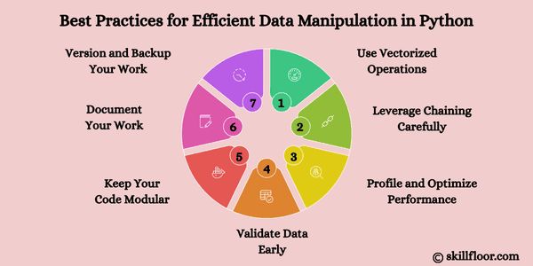
4. Validate Data Early

Always inspect data types, null values, and unique values before analysis:

print(df.info())

print(df.describe())

print(df.isnull().sum())

This prevents silent errors from propagating through your workflow.

5. Keep Your Code Modular

Break large scripts into reusable functions or pipelines. This enhances reusability and testing:

def preprocess(df):

    df = df.dropna()

    df['amount'] = df['price'] * df['quantity']

    return df

6. Document Your Work

Add comments and docstrings to describe what each block or function does. It helps future you (or teammates) understand the logic quickly.

7. Version and Backup Your Work

Use Git for version control. For datasets, store intermediary and final versions with clear naming and timestamps.

By incorporating these practices, your data manipulation projects in Python will become not only faster but also more robust, scalable, and easier to maintain. Whether you’re handling thousands or millions of records, structured workflows ensure long-term success.

Data manipulation is not just a technical task—it's a strategic skill that transforms raw, unstructured data into meaningful insights. In 2025, with data volumes at unprecedented levels, mastering Python's data manipulation capabilities is essential for anyone in the analytics, data science, or business intelligence fields.

From foundational operations like reading and cleaning data to more advanced topics such as time-series handling, text processing, and large-scale data management, this guide equips you with the knowledge and tools to take full control of your datasets. The libraries and techniques explored here are practical, versatile, and applicable to real-world scenarios across industries.

By following best practices and staying updated with the evolving ecosystem, you can ensure your data workflows are robust, reproducible, and efficient. Whether you’re working with small datasets in a local environment or scaling up with cloud-based big data tools, Python offers the flexibility and performance you need.