What is Gradient Descent in Machine Learning?

If you've ever tried to understand machine learning, you've probably reached that point where everything seems exciting and terrifying. You get the concept of model training. However, when someone says something like "gradient descent optimization algorithm," it's as if you've entered a world with a lot of mathematical processes.

Gradient descent isn’t just a formula or algorithm.

It’s the beating heart behind how AI learns.

The entire field of machine learning becomes much clearer, less difficult, and much more empowering to confidently navigate once you fully understand gradient descent in simple human words.

What Is Gradient Descent in Machine Learning?

Gradient descent is an effective optimization method that helps machine learning models learn from patterns, gradually reduce errors, and improve their performance over time.

Gradient descent functions as a guide when a model's predictions are not met, asking what went wrong and figuring out the best path for development.

Almost all contemporary machine learning systems, from simple regression models to massive deep learning models with billions of parameters and intricately linked layers, are powered by this technique.

In order to really comprehend gradient descent, we must investigate it both visually and emotionally, dissecting it into useful ideas that are easy to understand, intuitive, and actually significant to learn.

Why Gradient Descent Is Important

1. Guided Error Reduction

Gradient descent helps models improve accuracy through consistent, well-informed, step-by-step optimization by lowering prediction errors through parameter adjustments based on loss feedback.

2. Steady Model Improvement

Gradual performance improvements are made possible by this technique, which directs models to continuously improve parameters and generate predictions that are more significant, dependable, and accurate.

3. Efficient High-Dimensional Search

Through accurate gradient-based updates during training, gradient descent effectively traverses complicated high-dimensional spaces, assisting deep learning models in determining the best parameter directions.

4. Structured Learning Path

By restricting random parameter changes and guaranteeing that every modification brings the model closer to significant underlying data patterns, it creates a consistent learning direction.

5. Faster Training Cycles

Even with difficult datasets or large-scale designs, gradient descent uses directed gradients to speed up learning, allowing for quicker advancement and shorter training times.

6. Intelligent Self-Refinement

Models wouldn't improve intelligently without gradient descent; this method allows for ongoing improvement, allowing for dynamic forecasts rather than static, unchanging assumptions.

That’s gradient descent.

• The “mountain” = your error or loss function

• The “valley” = the optimal parameters

• Each “step” = adjusting parameters to reduce error

AI can learn patterns, make better predictions, and eventually surpass humans in some activities because of its capacity to "feel your way down the mountain."

Understanding the Intuition Behind Gradient Descent

• Sensing Error Direction: Gradient descent allows models to gradually "feel" which direction reduces errors and brings them closer to improved predicted performance by tracking how changing parameters impacts error.

• Following the Slope: Gradient descent follows the slope of the loss function and uses the steepest downward direction to identify the most promising improvement steps each iteration, as opposed to making random guesses.

• Blindfolded Descent Analogy: The intuition is similar to walking downhill while wearing a blindfold: you feel the slope of the earth beneath your feet and keep going down until you reach the lowest point.

• Gradient as Compass: By guiding the model in the direction of lower error, each gradient value functions as a compass needle, ensuring that training proceeds rationally rather than erratically over the parameter terrain.

• Controlled Learning Steps: Stable learning is made possible by small, controlled increments that prevent overshooting the minimum, while frequent tweaks steadily improve the model until error stops significantly declining.

  
  

• Continuous Parameter Refinement: By regularly adjusting parameters to reduce the overall value of the loss function, this methodical optimization enables models to learn intricate correlations and convert unprocessed data into accurate predictions.

A Step-by-Step Explanation of How Gradient Descent Works

Gradient Descent is a methodical and transparent approach to determine the optimal parameters and progressively lower the model's error. It learns by making numerous tweaks rather than attempting to get straight to the best solution. In the context of training machine learning models, this is an easy-to-understand, step-by-step explanation of how the algorithm operates:

1. Initialize the Parameters

The model's parameters (weights and biases) are first given random values during training. Gradient descent will gradually improve these, so they don't have to be perfect.

2. Make Predictions Using the Current Parameters

Based on the input data, the model predicts outputs using the initial parameters. At first, these predictions are typically very inaccurate.

3. Compute the Loss (Error)

A loss function, such as Mean Squared Error or Cross-Entropy Loss, is used to compare the anticipated and actual values. This shows the errors the present model is.

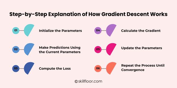
4. Calculate the Gradient

The gradient of the loss with respect to each parameter is then calculated by the method. The gradient indicates the direction of the loss's steepest increase, indicating that the way to its reduction is in the opposite direction.

5. Update the Parameters

Using the gradient and the learning rate (step size), the parameters are updated:

                                                      θ=θ−α⋅∂θ
                                                                 ∂L​

This step moves the parameters slightly downhill toward lower loss.

6. Repeat the Process Until Convergence

Steps 2 through 5 are repeated multiple times. Every cycle brings the parameters closer to the ideal values by slightly lowering the loss. This keeps happening until the loss stops getting better or the updates get very tiny.

Types of Gradient Descent (And Why They Matter to You)

1. Batch Gradient Descent

Batch Gradient Descent offers a stable and accurate approach to optimization, particularly in situations where accuracy is crucial. It achieves this by calculating the gradient using the entire dataset before updating the model's parameters.

This method results in smooth and predictable learning curves since all the data is processed simultaneously. It is particularly well-suited for smaller datasets or scenarios where CPU resources can easily handle large matrix operations.

However, this stability comes at the cost of speed; training can become more labor-intensive and slower. Understanding the importance of machine learning highlights why this method is preferred when precision is critical, despite being slower.

2. Stochastic Gradient Descent (SGD)

Using only one data point at a time, stochastic gradient descent updates parameters, resulting in a quick, dynamic learning process that continuously changes in response to instantaneous input from individual samples.

SGD is unexpectedly effective for complicated landscapes where smoother approaches could become stuck because of this quick mobility, which adds noise but also helps the model escape local minima more successfully.

The erratic learning pattern, which alternates between hurrying and stumbling, is almost emotional and reflects how people learn from each unique encounter while progressively improving their general comprehension.

3. Mini-Batch Gradient Descent

Mini-Batch Gradient Descent updates parameters using small batches of data, striking a balance that offers smoother gradient estimates and improved processing efficiency compared to purely stochastic methods.

This technique is particularly well-suited for large datasets used in contemporary deep learning training. It reduces noise without compromising speed, allowing models to learn efficiently without consuming excessive memory.

Often considered the "just right" option, Mini-Batch Gradient Descent combines momentum and stability, providing reliable updates that feel neither too chaotic nor too rigid during training.

The Role of the Learning Rate in Gradient Descent

One of the most important variables that affects how well gradient descent learns is the learning rate, often known as the step size. It regulates the size of the step the algorithm takes in each iteration to modify the model's parameters. The algorithm will descend smoothly toward the loss function's minimum if the correct learning rate is used.

Why the Learning Rate Matters

Gradient descent moves slowly when the learning rate is too low, resulting in incredibly slow improvements and longer training times, which frequently give the impression that the model is stationary.

An excessively high learning rate causes the algorithm to overshoot the minimum, resulting in unstable parameter updates that worsen the loss and unintentionally push training away.

The optimal balance between speed and stability is provided by a carefully selected learning rate, which enables gradient descent to converge effectively without producing unstable updates or erratic movements.

How the Learning Rate Affects the Path of Learning

• Small learning rate → smooth but slow descent

• Large learning rate → fast but potentially unstable movement

• Optimal learning rate → steady, efficient progress toward the minimum

In real-world applications, a lot of optimization algorithms dynamically modify the learning rate during training to enhance model performance, stability, and convergence speed.

Visualizing How Gradient Descent Works

• Loss Landscape Overview: The first step in visualizing gradient descent is to visualize a curved loss surface that represents the error values that the model continuously tries to reduce during training.

• Step-by-Step Movement: In order to reach areas with progressively smaller errors, each parameter update is similar to stepping downhill along the coast surface and following the slope direction.

• Gradient Direction Insight: The gradient, which takes the form of an upward arrow, shows how machine learning components inform the opposite movement required to lower mistakes.

• Learning Rate Effects: Learning rate diagrams illustrate how smaller steps preserve stability and direct optimization toward reducing error, whereas larger steps overshoot minima.

• Iterative Progress Visualization: Training plots demonstrate how the model is constantly guided downward by recurrent parameter changes, which progressively reduce error as optimization advances through learning iterations.

• Animated Descent Journey: The model descends the landscape in animated visualizations, displaying gradual refinement and smooth convergence driven by the selected learning rate.

Understanding the Challenges and Limitations of Gradient Descent

• Trapped in Minima: The model may not achieve the best global solution if gradient descent becomes trapped in local minima on complicated loss surfaces.

• Slow on Flat Areas: Small gradients produced by flat areas, plateaus, or saddle points result in incredibly slow progress and a substantial increase in training time.

• Learning Rate Sensitivity: Proper tuning is essential for steady training because a poorly selected learning rate may result in wild divergence or excruciatingly sluggish updates.

• Heavy Data Requirements: Gradient computations are computationally costly when dealing with large datasets, and batching techniques are frequently needed to preserve efficiency and training viability.

• Noisy Gradient Behavior: If stochastic gradient updates are not supported by sophisticated optimizers, noise may be introduced, leading to unstable movements and inconsistent training.

• Needs Differentiable Functions: Gradient descent is not directly applicable to models with discrete outputs or nondifferentiable operations since it requires differentiable loss functions.

Real-World Examples of Gradient Descent

1. Image Recognition Models (e.g., Google Photos, Face Unlock)

Gradient descent progressively lowers classification mistakes, which helps deep neural networks in learning to identify faces, objects, and scenes.

Every training repetition enhances accuracy—allowing apps like Google Photos, Instagram tagging, or smartphone face unlock to perform with incredible precision.

2. Recommendation Systems (e.g., Netflix, Amazon, Spotify)

Gradient descent is used by recommendation engines to precisely represent user-item interactions, which enables systems to improve predictions by reducing mistakes across a variety of watching, shopping, and listening patterns.

These systems continuously learn user preferences, increasing customisation, increasing engagement, and improving overall happiness across digital platforms by narrowing the gap between suggested and actually chosen content.

3. Language Models and Chatbots (e.g., ChatGPT, Siri, Translation Apps)

Large language models can comprehend context, syntax, semantics, and conversational purpose thanks to gradient descent, which iteratively lowers prediction errors across massive datasets.

Through ongoing learning advancements, this optimization process helps chatbots, interpreters, and voice assistants produce precise answers, preserve conversational flow, enhance clarity, and provide increasingly human-like interactions.

Best Practices for Using Gradient Descent Effectively

1. Tune Learning Rate Carefully

The model progresses effectively toward the minimum without overshooting or stalling during training when the right learning rate is chosen, preventing instability or sluggish progress.

2. Normalize Input Data

By prohibiting some characteristics from controlling updates, normalization or standardization lets gradients flow consistently, thus enhancing training stability, convergence speed, and overall model performance.

3. Use Mini-Batches Wisely

Mini-batch training is perfect for large datasets and deep neural network designs because it strikes a balance between gradient stability and computational efficiency, lowering noise while maintaining speed, demonstrating the practical value of machine learning methods.

4. Monitor Loss Consistently

Monitoring loss values during training facilitates the early detection of divergence, plateaus, or overfitting, allowing for prompt modifications that enhance accuracy, convergence behavior, and long-term model dependability.

5. Apply Advanced Optimizers

By smoothing updates and adaptively modifying learning rates, optimizers such as Adam, RMSProp, or Momentum speed up convergence and greatly increase training efficiency for complex models.

6. Implement Early Stopping

Early stopping ensures greater generalization on unknown data without needless iterations, protects models from overfitting, and stops training when improvements wane.

Final Thoughts: Gradient Descent Is More Human Than You Realize

In life, success rarely comes from one massive leap.

It comes from small, consistent adjustments.

Learn → Measure → Adjust → Repeat.

That’s gradient descent.

You'll achieve a degree of clarity and confidence that most people never attain if you genuinely accept it, both in machine learning and in your professional life.

You’re already taking steps.

This article is one of them.

Keep going.

Gradient descent is similar to learning how to ride a bike. Every step seems uneasy at first, and mistakes seem overwhelming. However, every little change you make teaches you something. Your progress will go more smoothly, and you'll feel more comfortable navigating the way ahead as you practice more. Comprehending Gradient Descent in Machine Learning makes challenging problems seem manageable by demonstrating how constant, steady progress results in significant advancement. The abilities you acquire here influence how you approach obstacles, resolve issues, and progressively get better in all aspects of your life—not just models and computations. Continue moving, trying new things, and having faith in the process.